3.1 Dataset

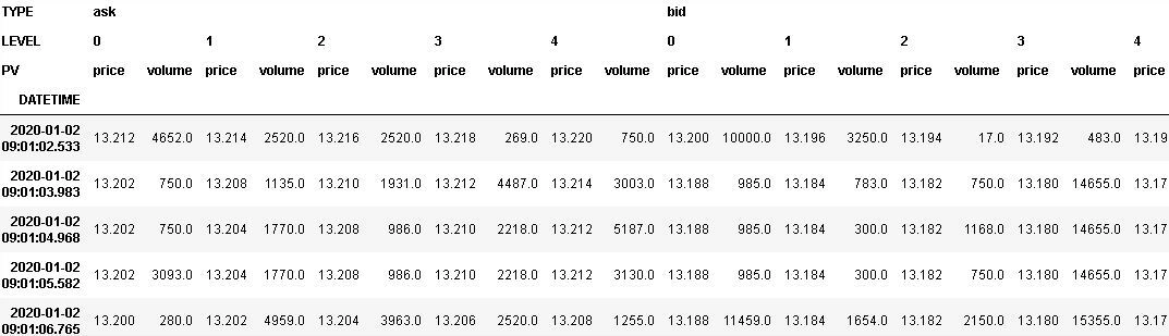
Our analysis has been performed on an extended set of stocks of the FTSE MIB index, in the period 1/1/2020-30/4/2020. The training set for the RL algorithm is constituted by the 1-second sampled FTSE MIB limit order book data of 2020, composed of five levels of prices and volumes for each side and each timestamp, and limited to the continuous trading period only. The figure here shows an extract from the book.

The test set is made up of the orders released by a “List customer specialist in equity markets” in 2020, of which we present a sample in the table below. Each of them has been split into a certain number of child orders as described in Sec. 2.1 of the previous post, following three different kinds of volume profiles between the order start and end times:

• the volume curve realised every day for the corresponding ISIN and measurable only at the end of the day, that is, a posteriori;
• the volume curve predicted by LIST for the corresponding stock and for every day;
• the green volume curve, namely, a curve identical for all the stocks and all the days.

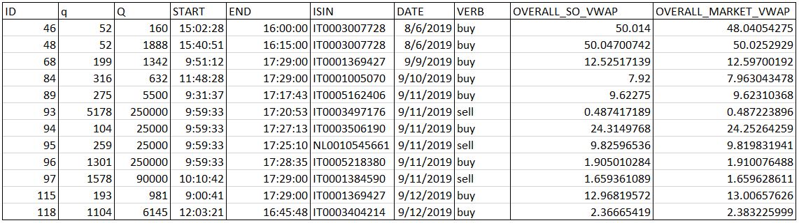
As displayed in the figure, the order features are: the client ID, the quantity $q$ to be executed in each interval, the total size $Q$, the start and end times, the ISIN, the date of execution, the verb (‘buy’ or ‘sell’), and the overall order and market VWAPs (which are respectively the one obtained by executing the LIST Smart Order between the order start and end times and the one derived from the market and calculated in the same period). The orders such that $q/Q > 0.5$ have been discarded. Moreover, if $Q$ is not a multiple of $q$, the quantity executed in the last interval is less than $q$.

3.2 NFK model

Below we present in detail the characteristics of our reinforcement learning model for optimal execution, the NFK model. The next sections are then dedicated to the description of the experiments carried out, with the specification of the methodology adopted, the algorithm implemented and the model parameter setting.

3.2.1 RL environment

The elements composing the environment in which our RL agent moves are listed below.

• States. The state variables are: the remaining time $t$, which represents how much time is left until the end of the horizon $H$, the remaining inventory $i$, which indicates how much volume is left to execute of the total quantity $V$, and the spread $s$, which is the current bid-ask spread with maximum value $S_{\rm max}$. For each stock analysed, we have performed a specific binning of the state variables, so as to find a compromise between including almost the entire ranges of values involved and limiting the computation time. With this in mind, the “resolutions”, i.e. the number of bins used for $t$ and $i$, are defined as $T$ and $I$, respectively.

• Actions. The action space is constituted by limit order prices, measured relatively to the current best ($ask$ or $bid$) price and expressed in tick sizes, at which we place our remaining shares. For the sell (buy) case, action $a$ means that we are repositioning all the unexecuted inventory at price $ask - a$ ($bid + a$) through a limit order. The action $a$ may be positive, signifying that we are “crossing the spread” towards the opposite side of the book, or negative, corresponding to placing the order within our own side of the book. Moreover, $a=0$ means that we are positioning our remaining shares at the current best price.

• Rewards. We have defined the immediate reward resulting from a certain action taken by the agent as the implementation shortfall (IS):

  $${\rm IS}=\pm \frac{\sum_{t=0}^{T}{q_t\cdot {\rm VWAP_t}} - q_{ex} \cdot M + 0.6 \cdot n_{exec}}{Q_0\cdot M}\times 10^4,$$

  where $q_t$ and ${\rm VWAP}_t$ are respectively the executed volume and the corresponding volume-weighted average price at time $t$, $q_{ex}$ is the quantity executed due to the action performed, $M$ is the mid-spread price ($(ask + bid)/2$) at the beginning of each episode, and $Q_0$ is the initial volume to be executed. The sign is added to take into account the verb ($+$ for buy, $-$ for sell). Furthermore, the term $0.6 \cdot n_{\rm exec}$ represents the cost deriving from the total number of executions $n_{\rm exec}$, being 0.6 euros the fee required by the market for each execution produced. This happens every time the book timestamp changes and/or the limit order matches a book level of the opposite side.

3.2.2 RL algorithm

The training algorithm is a sort of $Q$-learning and proceeds backwards in time, under the assumption that the actions of the RL agent do not affect the behavior of all the other market traders. This is ensured by the hypothesis of Markovian behavior of the system (see Puterman).

We have partitioned the training data into episodes, and we have divided every episode into a certain number of time bins with variable length (for the details, see the next section), with every bin consisting of intervals of 30 seconds each. At the beginning of each interval, the agent observes the state and submits a limit order (which is executed if its price meets the opposite side of the book), going on like this until it executes all the remaining quantity or reaches the end of the bin. If, after one or more bin “steps”, it gets to the end of the episode with some unexecuted shares, it then places a market order to force their execution.

In order to cover a wide range of values, we have randomly selected time and inventory within the relative bins, on a grid with a spacing of 30” and 50 shares respectively. For every episode, in every state encountered $s$, the RL agent tries every possible action $a$, which results in a reward $r(s, a)$ (computed as the sum of all the immediate rewards obtained through each 30” step) and brings the system to a new state $s’$. It also updates the expected reward $Q(s, a)$ deriving from taking each action and following the optimal policy subsequently, through the following rule:

$$Q(s, a) = Q(s, a) + \frac{1}{n(s, a)+1}\big[r(s, a) + \min_{a}Q(s', a) - Q(s, a)\big],$$

where $n(s, a)$ is the number of times that the agent has already tried action $a$ in state $s$. The $Q$-values are then written on a $Q$-table, which results in a (state $\times$ action) matrix.

For testing our RL strategy, we have divided the orders dataset into episodes, following the same method adopted for the training phase. Each episode is constituted by an order interval, where the quantity $q$ must be executed. Based on the trained $Q$-table, in every state encountered $s$, the agent selects the action $a$ giving the minimum $Q$-value in that state (if the sum of the matrix elements in correspondence of some state $s$ is zero, then the action is chosen randomly between the admissible ones), and uses this action to perform a bin “step”, which results in some executed quantity and realized countervalue. These values have been summed up to give quantity and countervalue relative to each interval, $q_{\rm int}$ and ${\rm ctv}_{\rm int}$, which in turn have been used to compute the volume-weighted average price for each order, ${\rm VWAP} = \sum {\rm ctv}_{\rm int}/\sum q_{\rm int}$, where the sums are all over the order intervals.

3.2.3 Parameter setting

The values of the tick size, and consequently of the bid-ask spread, along with the features of the orders concerned, depend on the particular stock and the specific time of the year. Therefore, periods with distinct tick sizes have been treated separately. The binning of the state variables and the set of actions have been defined as shown below:

• time bins (in minutes): [0, 1, 3, 6, 10, 30] ($T = 5$);
• inventory bins (in shares): [0, 1000, 5000] ($I = 2$);
• spread bins (in tick sizes): $[S_{\rm min}, …, S_{\rm max}]$, with at most 6 bins (the extreme bins $S_{\rm min}$ and $S_{\rm max}$ include multiple values, while the others contain single values);
• actions (in tick sizes): [-3, -1, 0, 1, 2], if $S_{\rm max} \leq 5$; [-5, -2, 0, 1, 3], if $S_{\rm max} > 5$.

As said before, we have performed the training/test distinguishing between the periods with different tick size and spread.

The training is performed on days taken at random between the start and end times of each period and not necessarily consecutive, in a number equal to the minimum between 50 (i.e. just over two months) and the total number of days (in case the period at hand has less than 50 days). The minimum number of training episodes is 500.

In the subsequent post we will present a preliminary analysis aimed at testing the capability of this reinforcement learning approach to handle the problem of optimal execution. Stay tuned!