2.1 HTM principles

Hierarchical Temporal Memory (HTM) is a biologically inspired machine intelligence technology, developed by NUMENTA, that mimics the architecture and processes of the neocortex. It is based on The Thousand Brains Theory of Intelligence (see A Framework for Intelligence and Cortical Function Based on Grid Cells in the Neocortex), which is a biological theory, meaning it is derived from neuroanatomy and neurophysiology and explains how the biological neocortex works. HTM principles are the technical details and algorithms that comprise the theory.

The HTM principles are the following.

• Common Algorithms: whatever is the problem to be analyzed, vision or hearing or text reading, the learning algorithms used by HTM are always the same.
• Sparse Distributed Representations: the representations used in HTM are called Sparse Distributed Representations, or SDRs. SDRs are vectors with thousands of bits, a small percentage of which are 1’s and the rest are 0’s.
• Sensory Encoders: HTM systems need the equivalent of sensory organs, which are called “encoders”. An encoder takes a certain type of data and turns it into a sparse distributed representation that can be used by the HTM learning algorithms.
• HTM Relies on Streaming Data and Sequence Memory: HTM learning algorithms are designed to work with sensor data that are constantly changing.
• On-line Learning: HTM systems learn continuously. With each change in the inputs the memory of the HTM system is updated.

2.2 Sparse Distributed Representation

The human neocortex is made up of roughly 16 billion neurons. The moment-to-moment state of the neocortex, which defines our perceptions and thoughts, is determined by which neurons are active at any point in time. One of the most remarkable observations about the neocortex is that the activity of neurons is sparse, meaning that only a small percentage of them are active at any point in time. The activities of neurons are like bits in a computer and so it is believed that the brain represents information using a method called Sparse Distributed Representations, or SDRs.

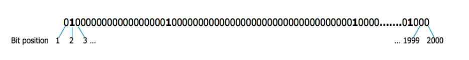
The SDRs used in HTM are binary representations consisting of thousands of bits where at any point in time a small percentage of the bits are 1’s and the rest are 0’s. Typically an SDR may have 2048 bits with 2% (or 40) being 1 and the rest 0. The bits in an SDR correspond to neurons in brain, a 1 being an active neuron and a 0 being an inactive neuron.

The most important property of SDRs is that each bit has semantic meaning. Therefore the meaning of a representation is distributed across all active bits.

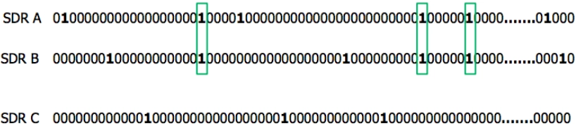This leads to the fact that two representations have similar semantic meaning if they share some of their active bits. In the image above we can see that SDR A and SDR B have matching 1 bits and therefore share semantic meaning. On the other hand SDR C does not share semantic meaning with the other two SDRs.

Another important property of SDRs is their robustness and the tolerance to error due to noise. The fact that the information carried by a representation is distributed among a small percentage of active bits means that flipping a single bits may not affect the overall meaning of the representation.

In case you are interested in learning about the other mathematical properties of SDRs we invite you to see Biological and Machine Intelligence (BAMI) digital book by Numenta.

2.3 Sensory Encoders

Any data that can be converted into an SDR can be used by HTM systems. Therefore, the first step of using an HTM system is to convert a data source into an SDR using an Encoder. There are some aspects to be taken into account when encoding data:

• Semantically similar data should result in SDRs with overlapping active bits.
• The same input data should always produce the same SDR as output.
• The output should have the same dimensionality (total number of bits) for all inputs.
• The output should have similar sparsity for all inputs (number of 1 bits).

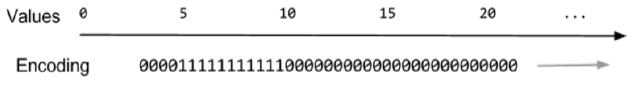
As an example consider a simple encoder for numbers. In this case we can encode overlapping ranges of real values as active bits. So the first bit may be active for the values 0 to 5, the next for 0.5 to 5.5, and so on. If we choose for our SDR to have 100 total bits, then the last bit will represent 49.5 to 54.5. The minimum and maximum values in this approach are fixed. The figure below shows the encoded representation of number 7.0 using an encoder with 100 bits, a value range per bit of 5.0 and an increase per bit of 0.5.

Other examples of encoders are described in Biological and Machine Intelligence (BAMI) digital book by Numenta.

2.4 Learning Algorithms

We will now briefly describe the learning algorithms behind an HTM system. For a more technical description of these concepts we recommend to access Biological and Machine Intelligence (BAMI) digital book by Numenta.

An HTM network is composed by a series of columns, each composed by cells. Each cell represents a bit that could be 1 or 0. The learning process consists of two steps, Spatial Pooling and Time Memory.

2.4.1 Spatial Pooling

The algorithm of Spatial Pooling permits to activate some of the columns of HTM network from the input data, which was previously translated into an SDR through an encoder. In other words it creates a new columnar SDR using the input data SDR. The Spatial Pooling algorithm has two important goals:

• it maintains a fixed sparsity, namely whatever is the sparsity of input SDR, the output will always have the same sparsity, i.e. the number of active cells will always be the same;
• it maintains overlap properties of input SDR, namely if two SDRs in input have similar semantic meaning, the Spatial Pooling will generate two output SDRs with overlapping active The HTM principles are the followingcolumns, in order to maintain the semantic similarity.

2.4.2 Time Memory

The next step of the learning process is the Time Memory. It has as input the SDR formed by Spatial Pooling. The Temporal Memory algorithm converts the columnar representation of the input into a new representation that includes state, or context, from the past. This is done by activating a subset of the cells within each active column, typically only one cell per column. By selecting different active cells in each active column, we can represent the exact same input differently in different contexts. The Time Memory algorithm also makes a prediction of what is likely to happen next. The prediction is based on the current representation, which includes also the context from all previous inputs.

In the next blog post we will show how to use the prediction made by the Time Memory layer in an anomaly detection context.