2.1 Dataset

As a testbed dataset for our analysis we have used a particular customer portfolio, partitioned by both underlying and expiry. This is because we intended to work with options on fixed underlying and not to include the Calendar Spreads, i.e. spreads in which the two options expire on different dates. In addition to this, we have performed tests on other types of portfolios with various sizes (i.e. the numbers of component positions), in order to better understand how the algorithm works when applied on a variety of collections of options. The figure below shows an extract of a typical input portfolio we have dealt with, which contains all the relevant options’ anagraphic data.

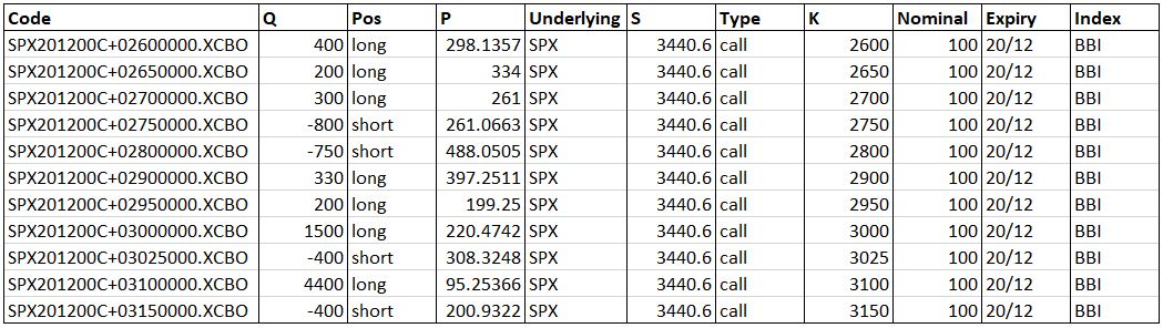
Here, Code is a peculiar characterization of the option, uniquely determined by its features. The option properties are: the quantity Q (positive for long and negative for short options), the price P, the strike price K, the Nominal face value, the position Pos (long/short) and the Type (call/put). Moreover, the option can be on Equity, ETF or index (Broad Based Index or Narrow Based Index), with the type of the underlying instrument affecting the margination formulas. The underlying price is instead given by S.

2.2 Algorithm

The algorithm we have implemented offers a heuristic approach to address the problem of minimizing the risk of a generic portfolio of options, by seeking for one or more collections of strategies aiming to produce the minimum margin for the portfolio. As said in the previous post, our proposed solution is a greedy algorithm of constructive primal heuristics (see De Giovanni).

The core of the algorithm begins by generating all possible significant strategies (1-leg to 4-leg) that can be built with the available options in a given portfolio and then selects a possible best-candidate among them, according to some tunable criteria. The options involved in such a strategy — namely, their involved quantities — are therefore removed from the original input portfolio, resulting in a new reduced portfolio from which to start again in a recursive approach that ends when no further strategies are available any more. The set of all the strategies selected on each recursion stage of this procedure represents a so-called scenario, of which the algorithm eventually computes the overall margin as the sum of the individual margins of the composing strategies. Implementing a multiple-choice strategy selection in the recursion core block allows to generate many different scenarios. In fact, our algorithm is capable to provide two distinct run modes:

• the one-shot mode, which corresponds to a “one recursion level, one choice” run and whose output may be regarded as the direct application of the strategy-selection criterion;
• the with-exploration mode, which instead entails a possible multiple choice on each recursion level, resulting in an exponentially growing amount of scenarios produced, among which the algorithm returns the lowest-margin one as the final output.

This has allowed us to make some benchmark analyses. Indeed, by selecting the one-shot criterion, we wanted to prioritize the algorithm performances over the solution optimality; instead, by choosing the with-exploration mode, we have been able to judge how much we got close to a better solution, although not exactly optimal.

2.3 Results

As we have examined a fair amount of different portfolios, the results obtained turn out to be specific for the inputs to which they refer and may vary appreciably from one to another. However, we have been able to formulate a certain number of considerations that are common to all the cases investigated and can take on, with good probability, the character of generality.

In particular, by analysing portfolios with various sizes, we could establish how exploration could improve the one-shot solution as the portfolio size changes. Of course, we expect that explorations lead to strategy-coverage configurations with a lower overall margin with respect to the one produced by the one-shot run, under the same simulation parameter values. Empirically, it turns out that exploration provides much room for improvement in the case of small portfolios, while this gain reduces as the size increases.

Look at the panel below.

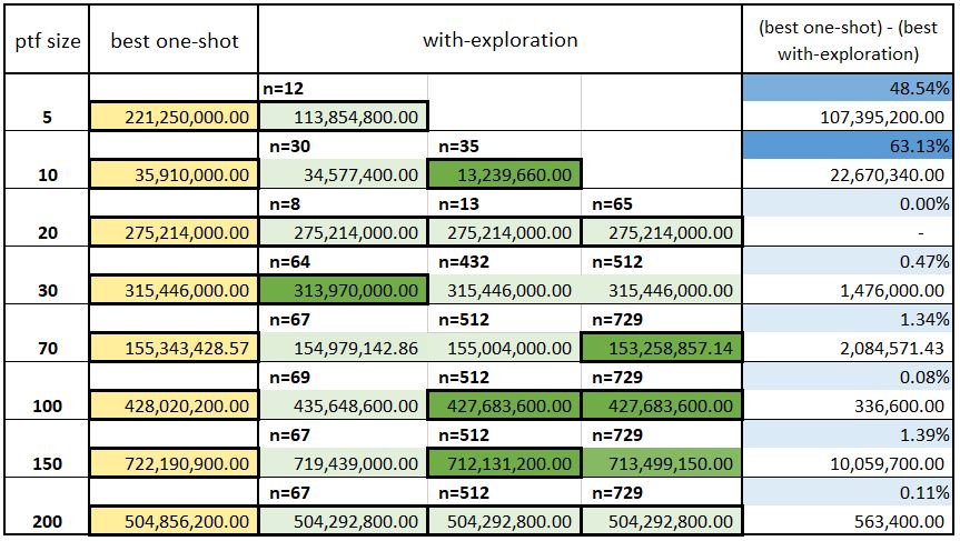
The figure exhibits the results of the application of our algorithm to a specific type of portfolio, of which we have varied the size from 5 to 200 (first column). The (best) outcomes of the corresponding one-shot runs are shown in the second column, while the third one contains the risk values produced through explorations with variable depth/width, where n represents the final number of configurations explored. Lastly, in the fourth column the (percentage and absolute) risk reductions produced by exploration over the relative best one-shot solution are presented.

Note that the values displayed in the figure, to be understood in currency, refer to the market risk and not to the initial margin. In fact, throughout our analysis we have assumed that the option premiums have been totally paid or received, thereby the net option value calculated for whatever sequence of strategies built from a given portfolio coincides with the one computed for the ensemble of the stand-alone starting options. Hence, we could detach the NOV from the calculation of the initial margin, and simplify our algorithm by focusing our attention on the sole MR term.

We notice that for portfolios with ${\scriptstyle\gtrsim}$ 20 options, the overall risk value obtained through exploration reduces on average by only few % units, at the cost of very long execution times. Conversely, exploration over portfolios with ${\scriptstyle\lesssim}$ 10 options may bring gains of up to ~70% and is not as time-consuming as the big-size case. It follows that, given the reduced amount of computing time and the noticeably high profits reached, doing exploration for small portfolios is convenient and can be easily performed exhaustively. Vice versa, the with-exploration solutions for large portfolios, as they are obtained at the cost of a high or very high computational time, can only represent super-optimal cases to be used as sort of benchmark. In fact, as the portfolio grows, the computing power needed to achieve meaningful results also increases. It is clear that, if in principle we were able to make extensive explorations, the resulting risks could be further reduced. Nevertheless, in such cases, even if no-exploration races cannot guarantee the optimality of the solution as a rule, they ultimately give reasonably acceptable results.

The most likely explanation for this empirical behavior is that the larger the portfolio, the smaller the region of the solution space the exploratory runs actually manage to explore, relative to the total number of possible combinations, which grows really fast as the size of the portfolio increases even a little. Moreover, to all appearances, the solution space must be extremely jagged and the probability of finding a solution that improves the value of the margin is probably somehow proportional to the volume of space explored, so it actually becomes exponentially smaller as the size of the portfolio increases.

So, on the one hand, with a small portfolio, even if the exploration logic does not proceed with small improvements, being able to fully explore the solution space eventually leads to finding the absolute minimum. On the other hand, for larger portfolios, a no-exploration run, which just directly applies one of the strategy-selection criteria we have identified as promising, already provides a competitive result, which evidently represents a local minimum compared to all other possible “close” alternatives.