4.1 Evaluation of a non-supervised learning RecSys

Since we are running a RecSys as anomaly detector, i.e. from a `bottom-up’ perspective, precision/recall at k metrics mentioned before are not much useful: we are not really interested in finding as many as possible interacted items among an as short as possible recommendation list.

Actually, if precedents of anomalous transactions were available, such traditional evaluation metrics for recommender systems like the Mean Average Precision could be employed by feeding them with the known-anomalous transactions and measuring how anomalous where scored by the RecSys. But this would be a case of supervised learning, where more direct approaches could be employed probably with better results with respect to a RecSys.

In any case, a generic score like the AUC value is nevertheless a good test for the classification performance of the calibrated model.

But even before that, we had to face a fitting convergence evaluation problem.

In fact, the calibration procedure consists in applying an iterative optimization algorithm with a loss function which somehow measures the difference between each interaction element (the rating, in case of explicit feedback) and the score returned by the RecSys. But since the ultimate purpose of a RecSys is not to truly forecast the users’ judgment, but just to rank the items for each user, an accurate agreement between the actual users’ rating and the returned numerical score value is a by far overkilling request. So, while the optimization algorithm in a generic curve fitting scenario is usually run up to some tolerance threshold on the loss function, in a RecSys framework it’s standard practice to just run it for a few step. This however leaves open the questions of when to consider a calibration procedure ‘settled’ and if the achieved calibrated model is meaningful whatsoever.

For this purpose we have adopted a self-consistency criterion, namely that different runs of the calibration procedure — with a different random seed but with the very same hyperparameter values, including the number of iterations to run — should generate models which give similar scores to available (user, item) pairs.

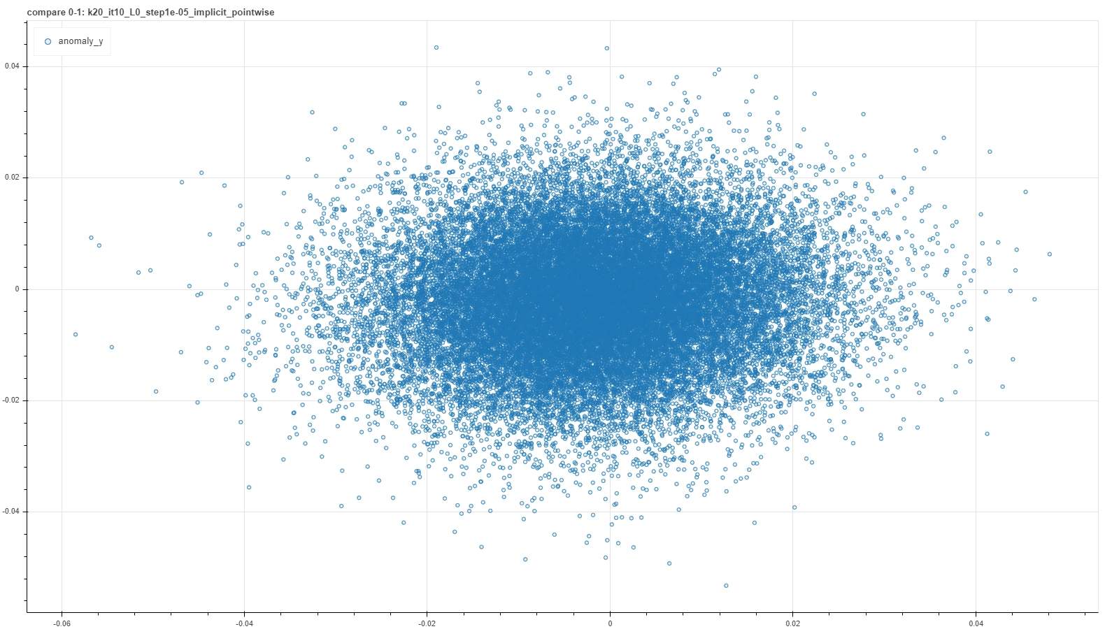
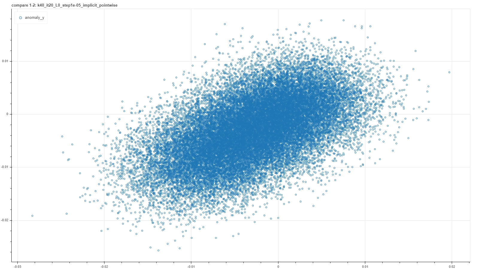
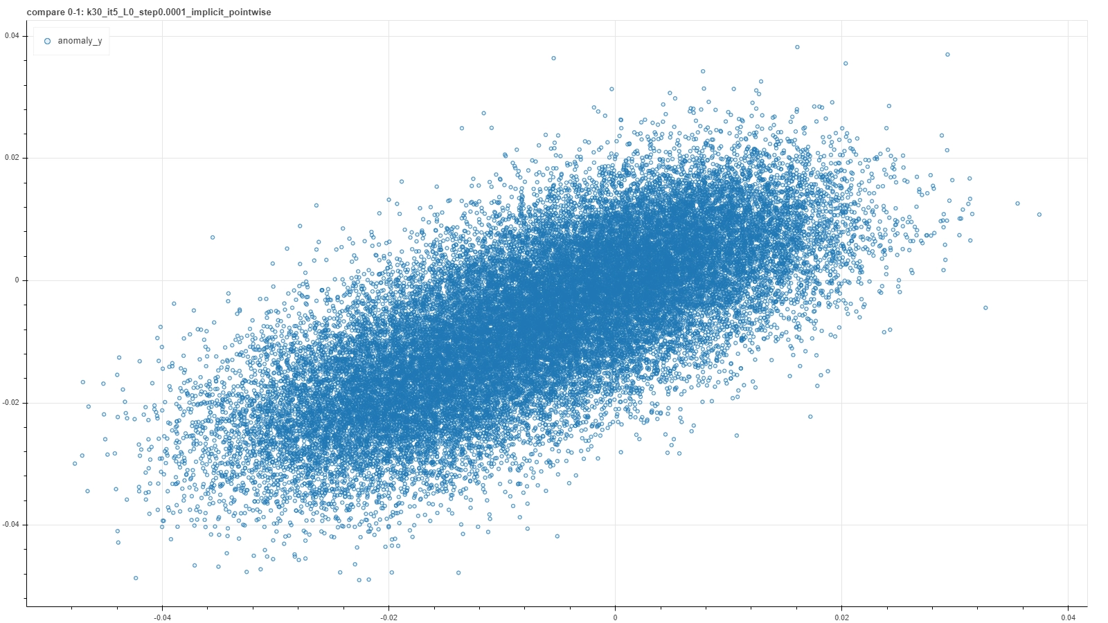
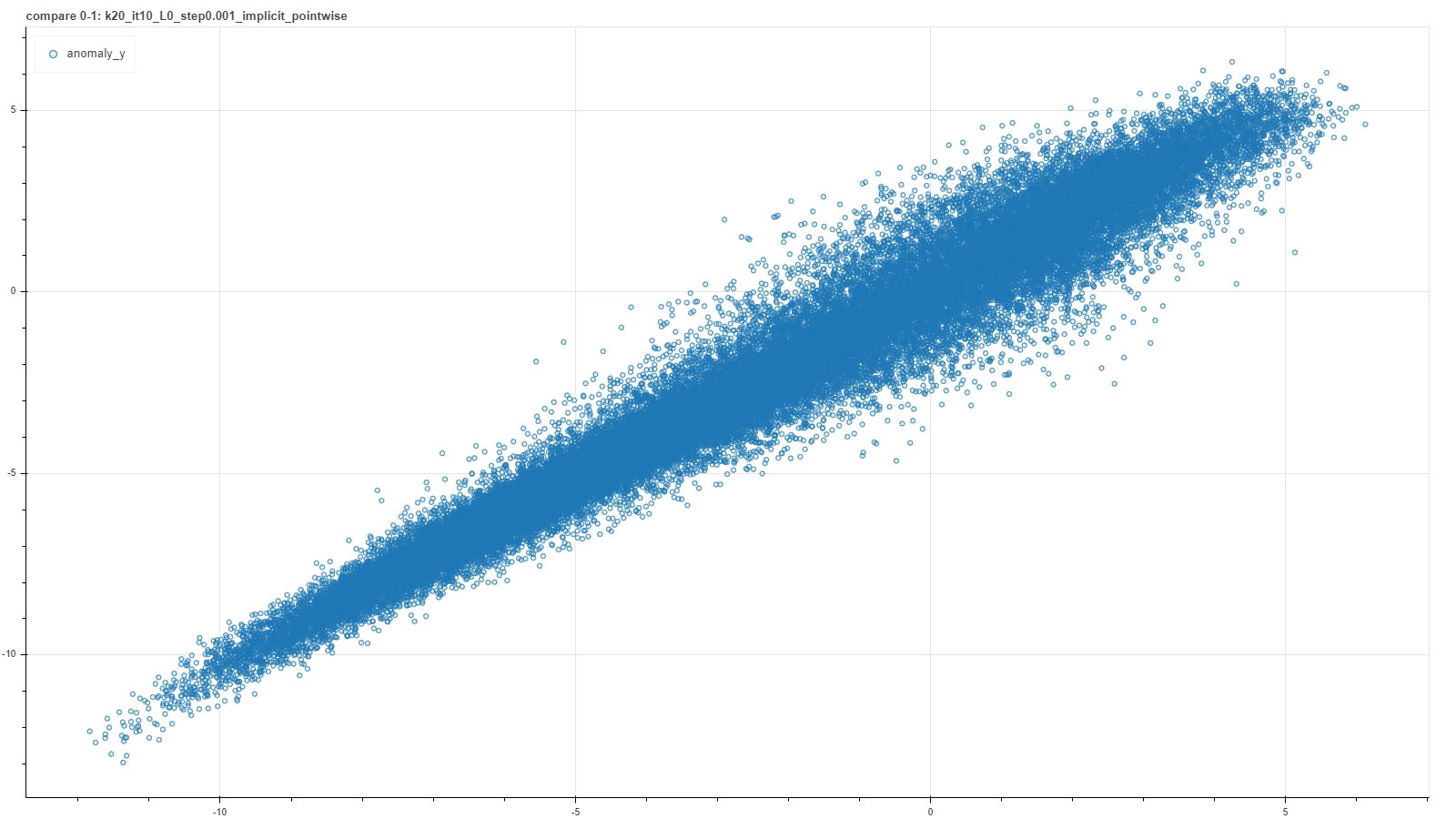
A visual representation of such a criterion can be found in a plot where score results from a couple of runs are plotted one against the other. In an ideal case of a deterministic result of the calibration procedure, each run would settle on the very same model and the plot would result in a perfect straight bisector line. In a more realistic but still good case, each calibration procedure would not reach exactly the same model, but nevertheless each of them would return similar score to the same pair. So the plot would result in a more blurred but yet bisector-like line.

A few examples of such plots are shown in the pictures below, where pairs of runs with the same hyperparameter values are captured in a single frame.

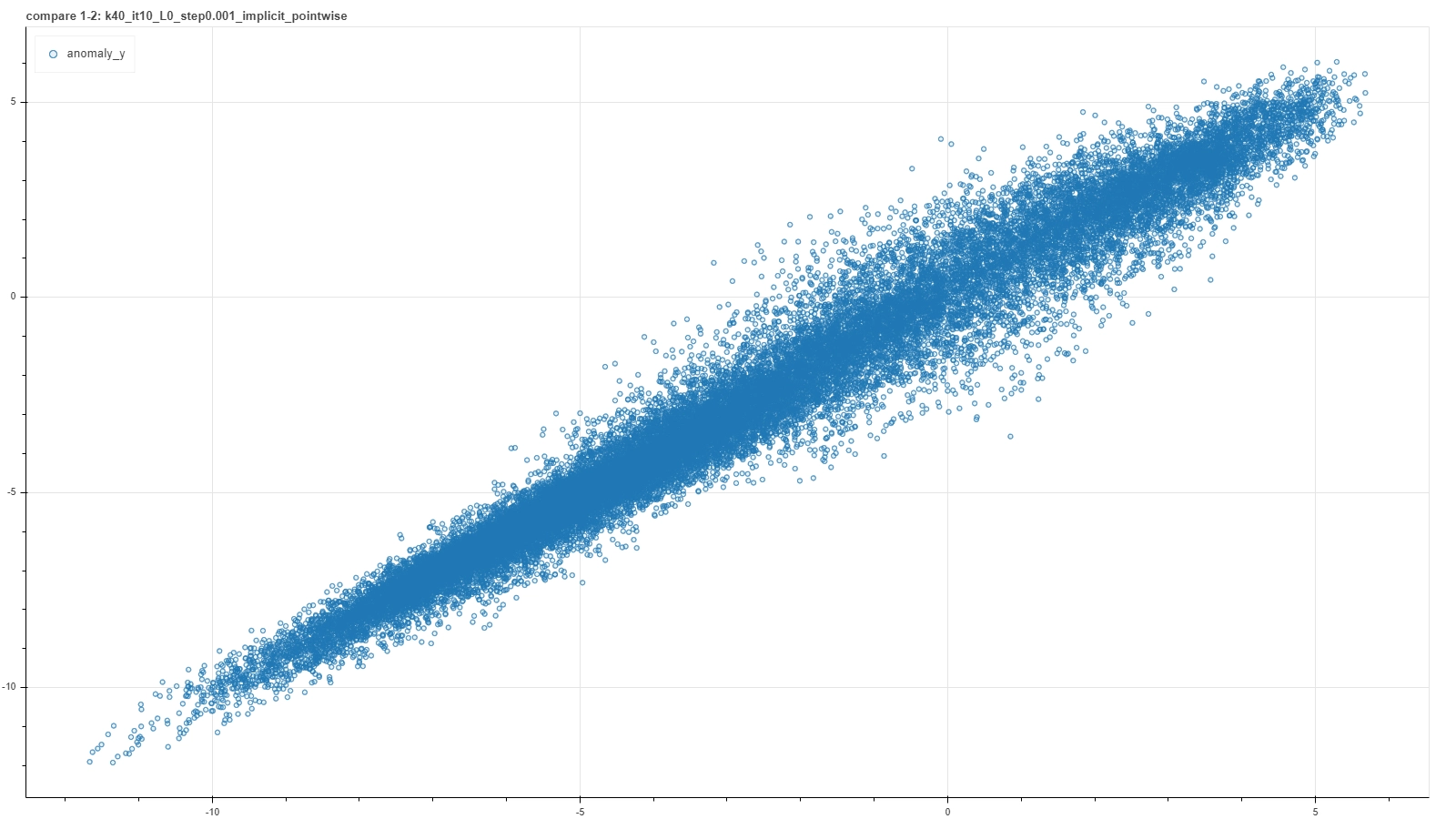From left to right and then from top to bottom the figures show gradually better situations. In each plot a single point represents a single deal and it’s placed at coordinates (x, y) based on the score returned by the RecSys calibrated in the first (x) and in the second (y) run with the same choice of hyperparameter values.

Notice that these plots do not represent intermediate steps along a single calibration procedure, but each is the outcome of a couple of iterative optimization runs for a specific — and completely different from one plot and the other — choice of hyperparameter values. Moreover, performing further optimization steps, for example for the first quite bad cases, generally does not improve the consistency, meaning that such particular arrangement of hyperparameters is just not adequate to capture features of the system.

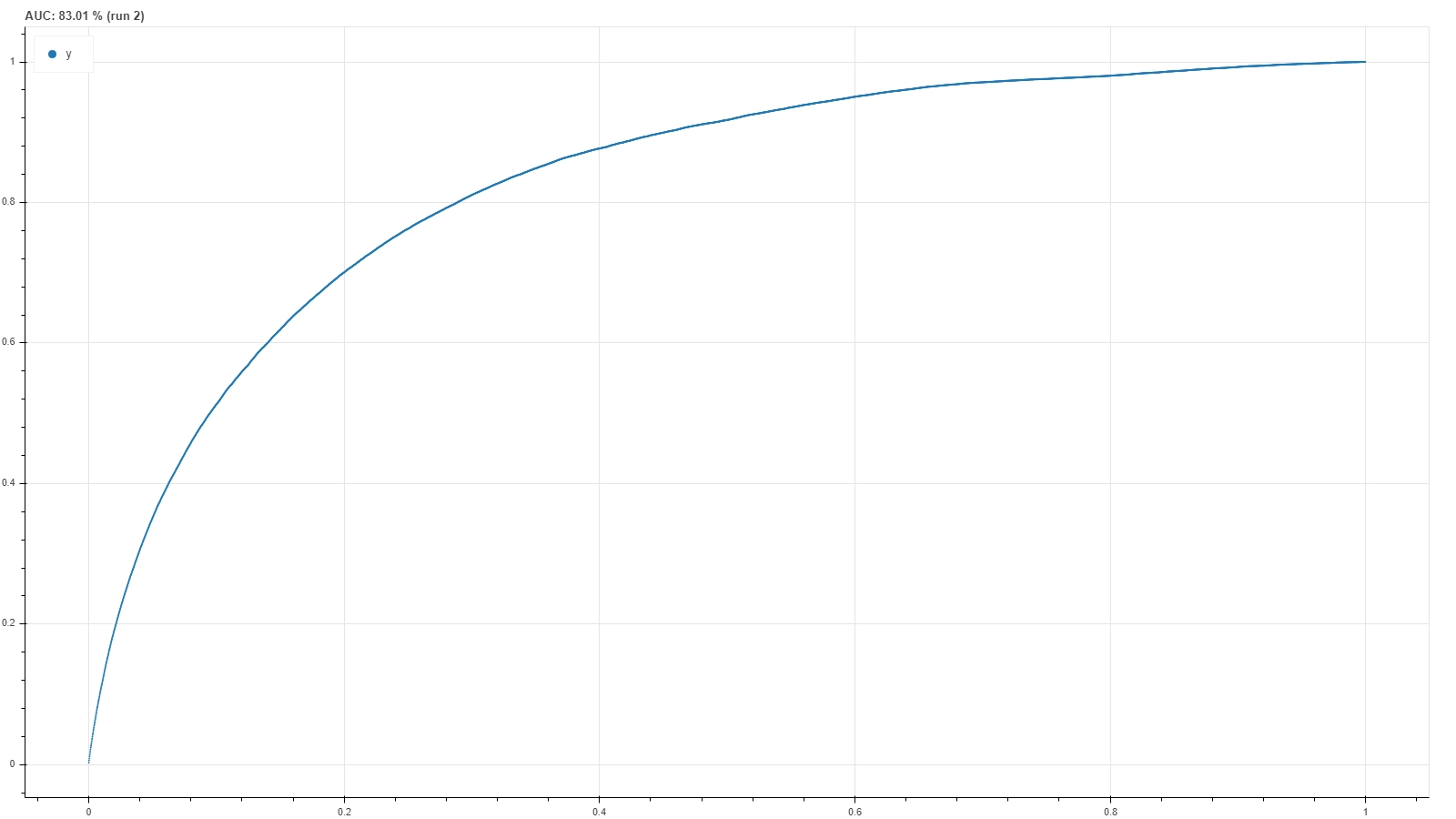Eventually, once gathered the most consistent hyperparameter configurations, one can further inspect their ROC curves and the corresponding AUC value to select the best configuration: see figure on the side for an example. It turns out, however, that the consistency condition is the stricter one: if, on the one hand, it happened that some ‘bad plot’ configurations still had a quite high AUC value, on the other hand all ‘good plot’ configurations performed well from the point of view of the AUC as well.