5.1 Score examples

One of the most important strengths of a RecSys approach is that it is able to assign a score even to users or items who have interacted little, if a sufficiently populated ovreall interaction sample is provided.

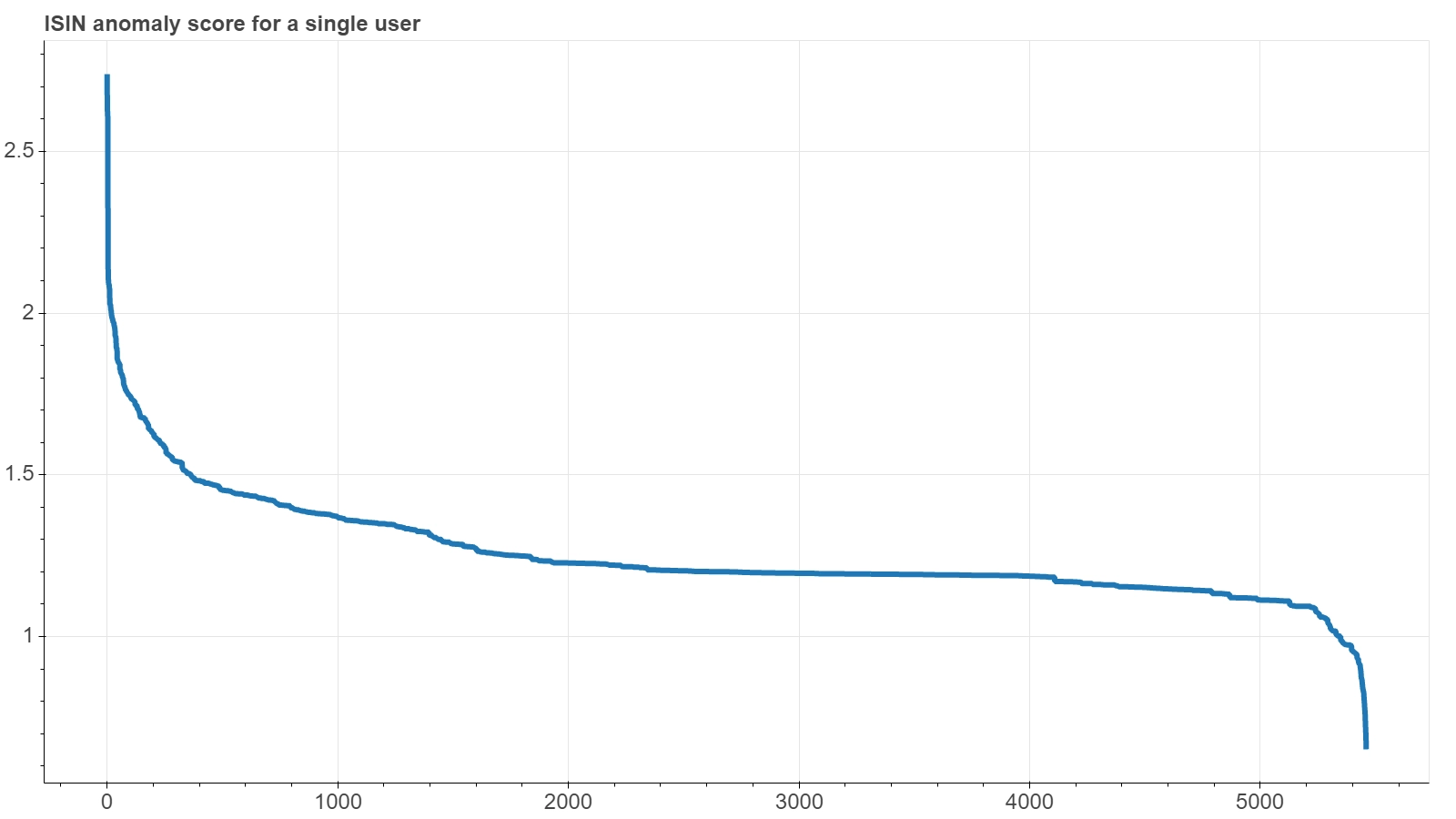A prime example is given by a plot like the one shown here, featuring a RecSys which uses the subject as the USER dimension and the security code (ISIN) as the ITEM dimension: all securities available in the dataset have been assigned have been given a score for a certain subject, not just the possibly small set of items she already dealt with in the training dataset. In the plot the items are sorted according to their score.

We already inverted the scale of the score with respect to the original output of a RecSys, so that we can directly read it as an anomaly score. Hence a lower value for an instrument means that the RecSys would recommended it for such a user, which in turns means that, if traded, it would be an interaction entirely consistent with that user’s typical behavior. On the other hand, a higher score would classify that instrument as highly anomalous, if dealt by that user.

As you can see, the RecSys highlights a rather small group of instruments as typical of that user: the ones with a higher rank, i.e. on the far right of the x-axis; then it classifies most of the instruments as ‘neutral’, the large central plateau: securities that are not specifically tailored for that user, but nonetheless plausible if traded by her; and finally it highlights a once again quite small group of instruments as ‘anomalous’, on the far left of the x-axis — what we are looking for.

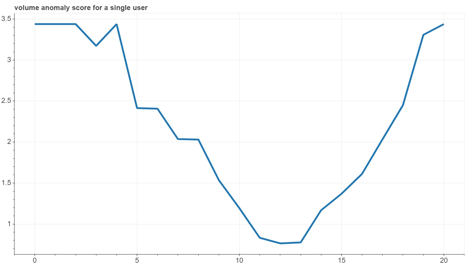The next figure shows the same plot for another RecSys, the one that uses the subject as the USER dimension and the countervalue of the transaction as the ITEM dimension. Actually here the items scored are the countervalues log-scale bins. In this case, since the ITEM dimension is not truly categorical and has its own metric, the bins were not sorted on the x-axis by the score, but were left in their natural order.

The plot clearly shows how the RecSys finds a quite definite countervalues region that it deems characteristic of the subject, since it increasingly judges as anomalous those bins that gradually move away from it, both on the left (smaller countervalues) and on the right (higher countervalues). The simple bell-shape of this output — which just resembles a vertical reflection of the histogram of the countervalues distribution — totally makes sense, since a quite natural pattern for each subject is just to have a main operating interval with increasingly reduced excursions moving away from that interval. It might also suggest that, in this particular case of an ITEM dimension with a proper metric, perhaps the same result could be obtained with a simple statistical analysis of the distribution of orders of each individual user. However, it should be borne in mind that not all users have a sufficiently large operation to allow to outline a countervalue profile from a single-user statistical analysis, while a RecSys approach can manage to sort out users looking at them as a whole.

5.2 Universal score reshaping

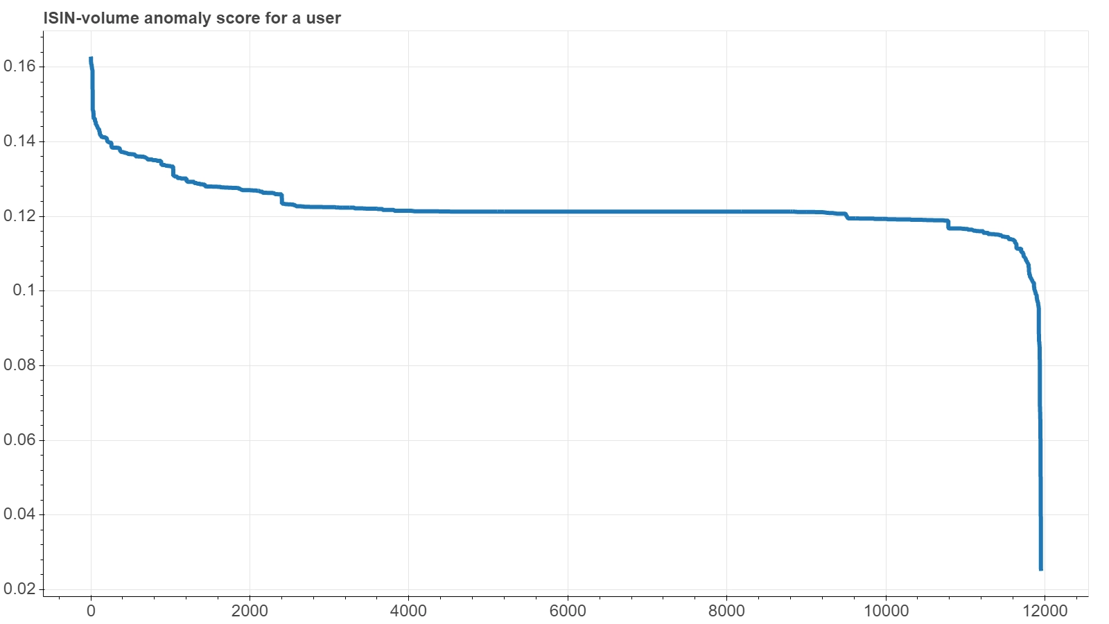The next figure shows the third example of an items-ranking plot for a single user, this time from the RecSys which uses a join of the ISIN and a per-subject volume-level as ITEM dimension.

As you can see, the y-axis scales of the last three plots are quite different from each other, since they reflect the details of the specific calibrated model. So, should a battery of RecSys-based anomaly detector tools be set up, specific alarm thresholds for each of them would be fine tuned.

A first naive normalization procedure could be to linearly rescale raw scores $\mathbf{s}_\mathtt{R}$ of each RecSys $\mathtt{R}$ into a normalized score $\mathbf{n}_\mathtt{R} = \dfrac{\mathbf{s}_\mathtt{R} - m}{M - m}$, where $M$ (respectively $m$) is the maximum (respectively minimum) raw value $\mathbf{s}_\mathtt{R}$ returned by each RecSys $\mathtt{R}$. In this way all the RecSys would return a normalized score $\mathbf{n}_\mathtt{R}$ that ranges between 0 and 1. But the problem of the different distributions of these values would remain: the plateau of the the first plot, for example, is much closer to the most anomaly values than that of the plot last plot, which instead is much closer to the opposite side. So, in these examples, the majority of pretty ordinary trades would be ranked with a much lower $\mathbf{n}_\mathtt{R}$ by the first RecSys with respect to what the last RecSys would return. Or, in other words, the middle point $0.5$ of such $\mathbf{n}_\mathtt{R}$ anomaly score would be a quite anomalous value if returned by the first RecSys, while it would definitely fall in the ‘recommended items’ region if returned by the last RecSys.

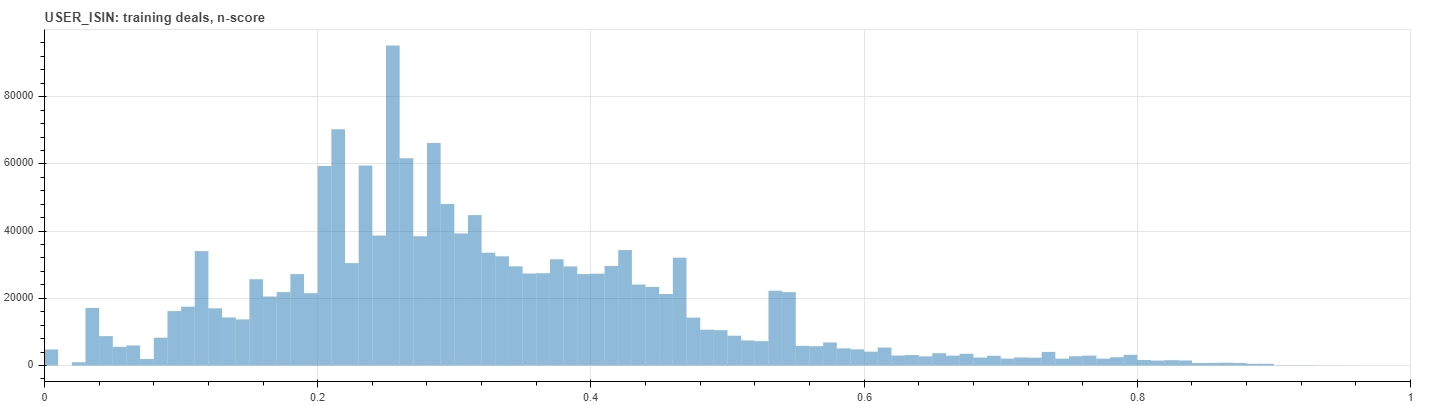
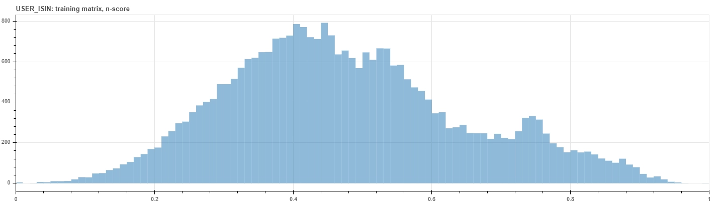
See for example the figures below that show the distributions of the normalized score within the training dataset. The upper histogram counts each deals on its own, while the bottom one counts just the interaction matrix elements. Notice that, due to the very definition of the rating metric, values lie mainly on the left of the upper histogram, since deals who occur often correspond usually to lower anomaly scores.

A possible way of overcoming such a variability is to convert each specific anomaly score into a universal z-score value, based on the distribution of the scores returned by each calibrated RecSys for the full interaction matrix. However, since generally these empirical distributions are not only not-Gaussian, but not even bell-shaped, we computed the z-score by means of the cumulative distribution function (CDF) of such distributions, rather than just by its mean and standard deviation. Actually we mapped the empirical CDF to the gaussian CDF:

$$\text{z-score} = CDF_{\text{normal}}^{-1}\big(CDF_{\text{empirical}}(\text{score})\big)$$

Using the quantile rank function $\mathcal{Q}_\mathtt{R}$ of the normalized score $\mathbf{n}_\mathtt{R}$ as a numerical proxy of the empirical CDF and by applying the inverse of the gaussian CDF, as usually denoted by $\Phi_{\mu,\sigma^2}$, with the standard parameters, namely zero mean $\mu=0$ and unitary variance $\sigma^2=1$, our z-score $z_R$ is given by:

$$\mathbf{z}_\mathtt{R}\, =\, \Phi_{0,1}^{-1} \big(\mathcal{Q}_\mathtt{R}(\mathbf{n}_\mathtt{R})\big) %_{\mu=0}^{\sigma=1}$$

This provides a universal way of representing an anomaly score, since it can be directly interpreted as the distance of a particular returned value from the mean of all possible scores, measured in terms of the width of the distributions of the scores themselves.

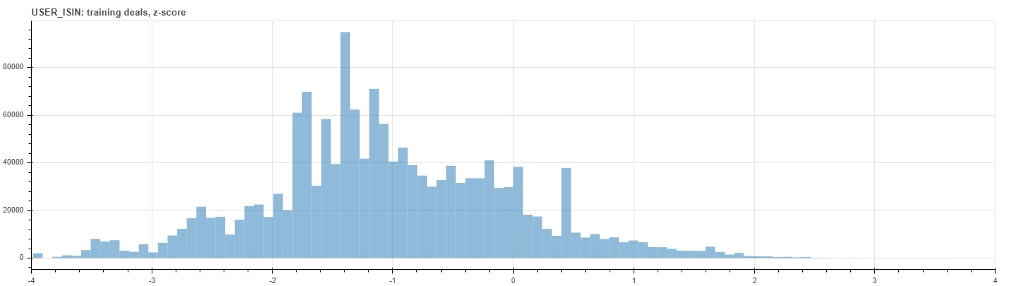
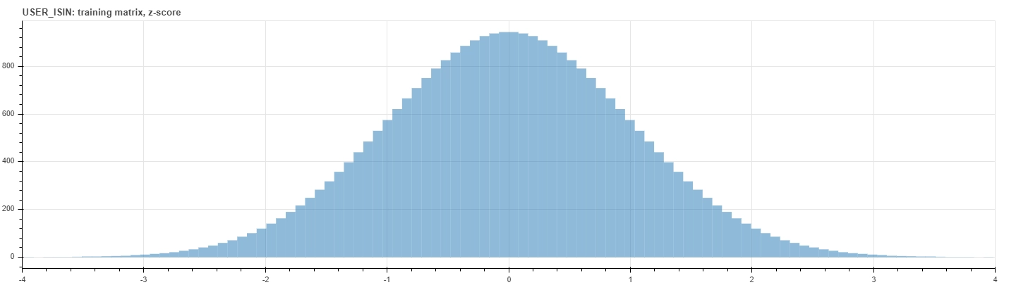
The last figures below show the distribution of the z-score within the training dataset. The upper histogram counts each deals on its own, while the bottom one counts just the interaction matrix elements. Notice that the latter is a perfect standard normal distribution by construction.