The dataset

We used the 360k alarms that are generated by a tier one Italian bank and already shown in the table 1 of the previous post. Those alarms have been generated with the LIST LookOut system that implements the MAR normative for the market abuse detection. LookOut accompanies every alarm with the pattern that has been violated and with a specific text that describes why that alarm has been raised. For instance, for an “Insider Trading” alarm the text is (we replaced the confidential parts with “date:time” and “name:surname”):
 

“Price sensitive information was published at date:time. The information was assessed as having a negative effect on the price (at least on MTAA), with a first over threshold price variation of -5.04% at date:time over the following days. This variation is greater than or equal to the 5% price variation threshold. ClientID (name:surname) amended, deleted or executed orders for a total gross value of 23040 in the 45 days preceding the public disclosure of the price sensitive news; in the 15 days preceding the news disclosure, the same entity operated for a total gross value of 23040, for a percentage of 100% of the entire gross value (above the 51% threshold). In the period between date:time and date:time, the ratio between net (-23040) and gross (23040) value was 100%, above the threshold of 51%, indicating a positive impact on the financial position of the analyzed entity. The net value was -23040, above the Minimum value of orders/trades threshold set to 10000.”

  After splitting all the fixed sentences parts from the “alarm-specific values” present in the text, it can be translated in a field/value table of this kind:

field	value
user	ClientID (name:surname)
Price_sensitive_information_published_at	date:time
The_information_assessed_as_having_a	negative
effect_on_the_price_at_least_on	MTAA
with_a_first_over_threshold_price_variation_of	-5.04
at	date:time
over_the_following_days_This_variation_is_grea...	5
price_variation_threshold_@@@_amended_deleted_...	23040
in_the	45
days_preceding_the_public_disclosure_of_the_pr...	15
days_preceding_the_news_disclosure_the_same_en...	23040
for_a_percentage_of	100
of_the_entire_gross_value_above_the	51
threshold_In_the_period_between	date:time
and	date:time
the_ratio_between_net	-23040
and_gross	23040
value	100
above_the_threshold_of	51
indicating_a	positive
impact_on_the_financial_position_of_the_analyz...	-23040
above_the_Minimum_value_of_orders/trades_thres...	10000

We performed this translation for all the alarms obtaining for “Insider Trading” a set of 68719 tables of the previous kind. All the tables of the insider trading have the same list of 22 fields since the structure of the alert message is the same. So, we can transpose and merge all the 68719 tables obtaining a unique dataset for the insider trading of 68719 rows, that is one row for each alarm, and 22 fields. Associated with this dataset, that represents the inputs to the ML, we have also an array of 68719 classification status belonging to the two classes: Closed or Signaled.

With this dataset, we are ready to apply the training of the ML methods for the insider trading. We can repeat the same pre-processing of the alarms also for the other patterns to obtain a specific dataset for each of them.

Imbalance

As already said in the previous post the dataset is heavy imbalanced: in fact, the insider trading pattern has 99.6% of the alarms belonging to the class Closed (68442 Closed and only 277 Signaled). Ignoring the imbalance problem would result in a trained ML agent capable of a high accuracy (at least 99.6%). In this way, when queried to classify a new alarm, it would just answer “Closed” all the time, but it would not be able to recognize any of the few alarms to be Signaled.

We tried different ML methods, but we finally choose the Random Forest (RFA) since it offers more methods to deal with the imbalance. These methods can be classified in two different approaches:

Over-sampling

It consist in artificially increasing the minority class until the number of the two classes are homogeneous. Among these we can find:

• Naive random over-sampling,
• Synthetic Minority Oversampling Technique (SMOTE),
• Adaptive Synthetic (ADASYN),
• their variants

Under-sampling

It consists in artificially decreasing the majority class until the number of the two classes are homogeneous. One has to pay attention not to reduce too much the dataset applying the under-sampling, because she risks losing the learning capacity of the algorithm. Among these:

• Naive random under-sampling,
• Controlled under-sampling with different methods: Tomek’s link, Nearest Neighbors, and so on…

It is out of scope to describe the theory underlying these techniques, please refer to the documentation of the Imbalance-Learn Python package if you are interested. This package is the same that we used in our training experiments. We found that the choice of the imbalance technique to be used depends on the pattern. For some of them the over-sampling performs better and for others is the under-sampling instead. Anyway, we found that the naive random methods (under or over) are enough to achieve good results.

How to measure the results of the ML algorithm

In the context of binary classification three concepts are important:
The ‘population’, that is how all the cases are distributed between the two classes. In our case, from the table 1 of the previous post, we know that for insider trading the binary distribution is 99.6% Closed and 0.4% Signaled.
The ‘effectiveness of the test’, that is how much a test is able to say that an alarm is of class x when we already know that it is x.
The ‘prediction ability of the test’, that is, given a case that we don’t know which class it belongs to, the capacity of the test to predict the right class.

In our analysis, the test is a Random Forest Classificator, but you will find these concepts in all the medical test. Think, for instance, to the Covid-19. Nowadays we have at our disposal two tests: the rapid and the molecular. We know from the empirical evidence that the molecular is much more effective than the rapid, that is: on 100 infected people that submit the two tests the molecular recognize the infection in many more people than the rapid.
But when you go to a pharmacy to make the Covid-19 test you don’t know if you are infected or not! Once you receive the verdict, you may also be interested to know the probability that this judgment is correct or not. This last information is exactly the ‘prediction ability’ of the test and it is different from the information regarding the effectiveness.
Let’s see how to calculate practically these measures.

Effectiveness of the test

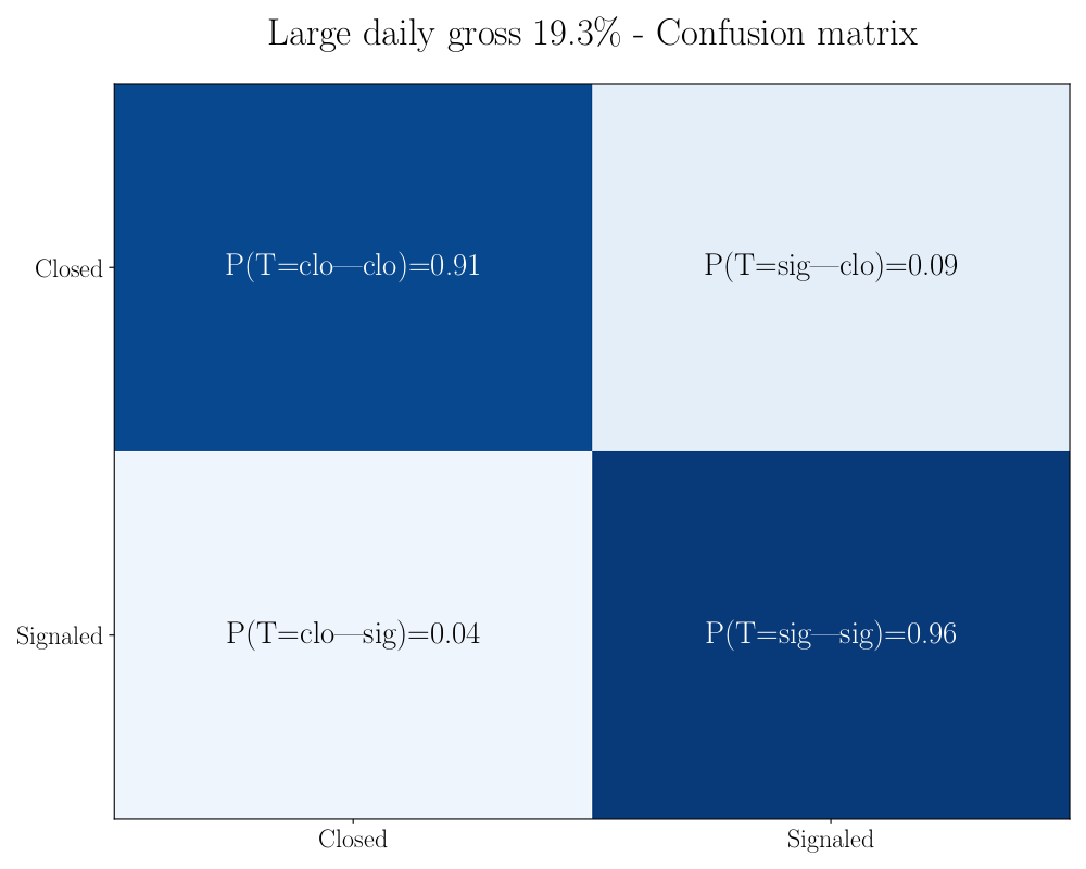It is measured by the so called ‘Confusion Matrix’, a square box in which on the rows there are the true distribution of the classes in the test and on the columns the predicted classes. Here an example for the ‘Large Daily Gross’ pattern. You can see that the frequency that the test gives Closed when the alarms was effectively Closed is 91% with only 9% of failure. This failures are the RFA false positive because on actually closed alarms the RFA said that have to be signaled. Viceversa on actually signaled alarms the RFA has 96% frequency to guess and only 4% of failure. These failure are the false negative.
 

 
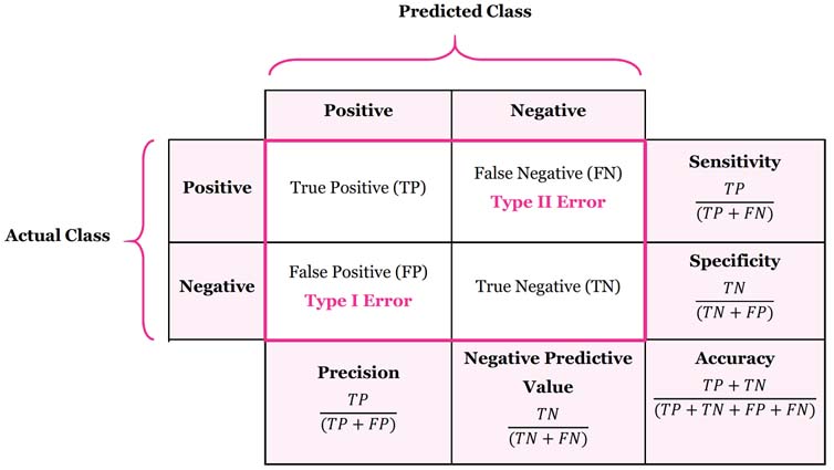
 The standard metrics used in binary classification to judge the effectiveness of a test like: Precision, Recall, Prevalence, Sensitivity, Specificity, F1-Score, are calculated starting from the values in the confusion matrix, as in the side picture.

 

Prediction ability of the test

As we saw before, it is the probability of the test to provide the right classification. That are: $P(clo|RFA=clo)$ and $P(sig|RFA=sig)$.

As counterpoint we have also the probability of being wrong, that are simply: $P(sig|RFA=clo)= 1-P(clo|RFA=clo) $ and $P(clo|RFA=sig)=1-P(sig|RFA=sig)$.

What counts for us in our context is to have a small $P(signaled|RFA=closed)$ because this is the error that produce the most severe effects with the Regulator since it coincides with a missing reporting. This probability can be computed with the Bayes Theorem:

$P(sig|RFA=clo)=\dfrac{P(RFA=clo|sig)\times P(sig)}{P(RFA=clo)}$

with:

$P(RFA=clo)=1-P(RFA=sig)=1-P(sig)\times P(RFA=sig|sig)-P(clo)\times P(RFA=sig|clo)$

Two metrics for the results

We introduce two metrics that allow to judge in a quantitative way whether the RFA will be useful for our final goal. The first metric we call it RISK. It is a measure of the probability to miss reporting to the Regulator a market abuse because the ML algorithm RFA told us to close the related alarm. The second metric is the WORK. This is a measure of how many residual alarms are left to check by the compliance officer if she allows the RFA to close automatically all the alarms that are classified to be closed. With these two metrics, we can have a more practice and human readable overview of the RFA performances. In fact, the WORK tells how many alarms are left to check, and the RISK tells how many market abuses we miss reporting.

Let’s start to define formally the WORK. It is simply the number of alarms for which the RFA tells to be signaled. In fact, trusting the RFA, all the alarms for which it tells to be closed will be automatically closed so only those with $RFA=signaled$ will be left. Formally the work left for 1000 alarms generated by the MAD System is:

$WORK=1000\times P(RFA=sig)$.

The RISK for one thousand of alarms is formally defined as:

$RISK=1000\times P(RFA=clo)\times P(sig|RFA=clo)$

 

 

Let’s clarify with an example for the Large Daily Gross (LDG).
From the population of the LDG, represented in the table 1 of the previous post, we can take:

$P(clo)=\dfrac{69855}{70032}=99.75\%$
 

$P(sig)=\dfrac{125+52}{70032}=0.25\%$
 

Then suppose that, after the training of the RFA, on the testing set that consist of 10000 alarms, the RFA gives the following confusion matrix
 

	pred Closed	pred Signaled
true Closed	9077	898
true Signaled	1	24

 from which we can take these probabilities:
 

$P(RFA=sig)=0.25\% \dfrac{24}{25}+99.75\% \dfrac{898}{898+9077}=9.22\%$
 

$P(RFA=clo)=1-P(RFA=sig)=90.78\%$
 

$P(RFA=clo|sig)=\dfrac{1}{25}=4\%$
 

With the Bayes theorem we can compute, in case of ‘closed’ response, the probability of wrong classification:
 

$P(sig|RFA=closed)=\dfrac{4\%\times 0.25\%}{90.78\%}=0.011\%$
 

and finally compute the WORK and the RISK for 1000 alarms:
 

$WORK=1000\times 9.22\%=92.2$
 

$RISK=1000\times 90.78\%\times 0.011\%=0.0998$
 

That is: without applying the ML algorithm the compliance officer has to check manually 1000 LDG alarms. Instead, with the help of the ML, the RFA will close automatically 908 alarms and she has to check manually only 92 alarms. The cost she has to pay for this saving of manual work is the risk to miss one market abuse every $\frac{1000}{0.0998}=10014$ alarms. Looks good, doesn’t it?

 

What presented here is just an example with invented numbers, that has been provided for a better comprehension of the metrics used to evaluate the performance of the RFA. The actual results of the RFA on the real dataset will be presented in the next post, so don’t miss the next episode!